Modeling and Accessing Relational Data

Part 2 in a series on the basics of the relational database and SQL

November/December 2011

Part 1 in this series, “Get Your Information in Order” (Oracle Magazine, September/October 2011), introduced readers to relational databases and the language chiefly used to interact with them: structured query language (SQL). Building on the material I presented in Part 1, this article explains relationship concepts in more depth and outlines the process of designing a new database. Then it introduces you to three tools available at no charge that you can use for viewing and managing the data in an Oracle Database instance via SQL. (Although I’ll briefly review the concepts covered in Part 1, I encourage you to read that installment before starting this one.)

Data is organized in a relational database as tables—two-dimensional matrices made up of columns and rows. A table’s primary key, enforced by a primary key constraint (which will be defined in a future article in this series), is a column or combination of columns that ensures that every row in a table is uniquely identified. Two tables that have a common column are said to have a relationship between them; the common column is the foreign key in one table and the primary key in the other. The value (if any) stored in a row/column combination is a data element.

The cardinality of a relationship is the ratio of the number (also called occurrences) of data elements in two tables’ related column(s). Relationship cardinality can be of three types: one-to-many, one- to-one, or many-to-many.

One-to-many (1:M). The most common type of relationship cardinality is a 1:M relationship. Consider the relationship between the EMPLOYEE and DEPARTMENT tables shown in Figure 1. The common column is DEPARTMENT_ID (which is the primary key in the DEPARTMENT table and the foreign key in the EMPLOYEE table). One individual DEPARTMENT_ID can relate to many rows in the EMPLOYEE table. This represents the business rule that one department can relate to one or many employees (or even no employees) and that an employee is associated with only one department (or, in some cases, no department). This business rule can be restated as follows: Each employee in a department may be in one and only one department, and that department must exist in the department table.

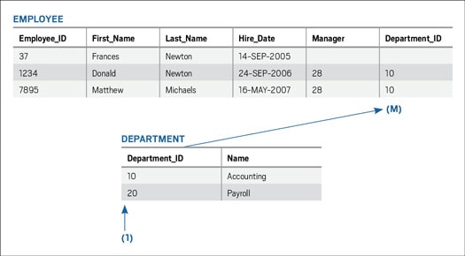
Figure 1: EMPLOYEE and DEPARTMENT tables with a 1:M relationship

One-to-one (1:1). A 1:1 relationship between the DEPARTMENT table and the MANAGER table is depicted in Figure 2. For every row in the DEPARTMENT table, only one matching row exists in the MANAGER table. Expressing this as a business rule: Every department has at least one and at most one manager, and, conversely, each manager is assigned to at least one and at most one department.

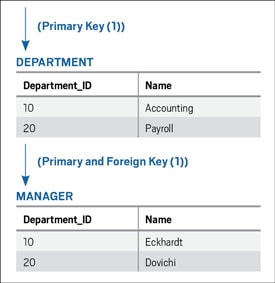
Figure 2: DEPARTMENT and MANAGER tables with a 1:1 relationship

One-to-one data relationships can exist, but they are not typically implemented as two tables (though they may be modeled that way). Instead, the data is combined into one table for the sake of simplicity.

Many-to-many (M:M). Consider the EMPLOYEE and PROJECT tables in Figure 3. The business rule is as follows: One employee can be assigned to multiple projects, and one project can be supported by multiple employees. Therefore, it is necessary to create an M:M relationship to link these two tables.

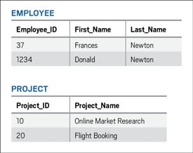
Figure 3: EMPLOYEE and PROJECT tables requiring an M:M relationship

To support the relational database model, an M:M relationship must be resolved into 1:M relationships. Figure 4 illustrates this resolution with the creation of an associative table (also sometimes called an intermediate or intersection table) named EMPLOYEE_PROJECT.

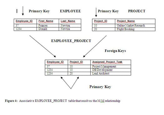
Figure 4: Associative EMPLOYEE_PROJECT table that resolves the M:M relationship

In this example, the associative table’s primary key—a composite of its Employee_ID and Project_ID columns—is foreign-key-linked to the tables for which it is resolving an M:M relationship. It reflects that one employee can be assigned to multiple projects—and, in this example, that one employee can be assigned multiple and different responsibilities for each project to which that person is assigned. Note that the employee with an EMPLOYEE_ID value of 1234 is assigned to two projects but that his responsibilities are different for each project.

For conceptual purposes, it is helpful to display table relationships of different types by using database schema diagrams. (A schema is typically a grouping of objects, such as tables, that serve a similar business function.) Schema diagrams—also known as physical data models—can use several types of standard notation. The schema diagram in Figure 5 uses a convention called crow’s-foot notation—the standard notation used by Oracle SQL Developer Data Modeler, a database modeling and design tool. With crow’s-foot notation, a crow’s foot, or fork, indicates the “many” side of the relationship and a single line with an arrowhead indicates the “1” side of the relationship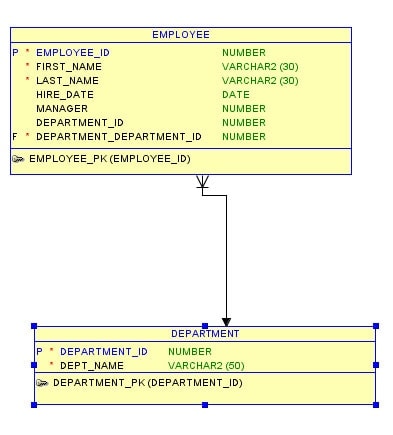
Figure 5: A database schema diagram showing a mandatory foreign key relationship between the EMPLOYEE and DEPARTMENT tables

The schema diagram in Figure 5 shows a mandatory relationship between the EMPLOYEE table and the DEPARTMENT table. A mandatory relationship—indicated by the solid line between the crow’s foot and the arrowhead—is one in which a value must be present in a foreign key column. In Figure 5, this means that every employee must be assigned to at most one department and at least one department. If the relationship were optional, the relationship line would be dotted instead of solid, indicating that an employee can be assigned to one or no department. (In Figure 5, the P in the left margin indicates the primary key, and the F indicates a foreign key.)

Before developers, DBAs, or database architects create tables—or even schema diagrams—they gather data requirements that identify the needs of the system users. Among other things, requirements gathering should result in a list of individual data elements the users consider important and need to store. The developer or DBA then groups what the users consider to be the most important data elements in this list into entities. The individual data elements are known as the entities’ attributes.

This creation of entities and their attributes, along with the necessary entity relationships based on business rules, is often referred to as logical data modeling. It is “logical” because it doesn’t take into consideration a specific technical (or physical) implementation. Entity is the logical term for a physical implementation’s table. And attribute (or, sometimes, field) is the logical term for column. A diagram depicting a logical data model is known as an entity-relational diagram (ERD). Specialized tools such as Oracle SQL Developer Data Modeler facilitate the generation of ERDs.

After you have created a logical data model and chosen your physical technical implementation, such as Oracle Database 11g, you are ready to create your database schema diagram (the physical model). When you create the schema diagram, you assign a datatype to each of your tables’ columns. The datatype specifies the type of data (such as numeric, character, or date) that can be stored in each column.

Data normalization is the process, based on widely accepted rules, that developers and DBAs use for tables to eliminate redundancy from data. Conversely, denormalization is the act of adding redundancy to data. When designing a physical database model, database designers must weigh the advantages of eliminating all redundancy—resulting in data that is split into many tables—against possible reduced query (data retrieval) performance when some or many of these tables are joined together via SQL. (You’ll learn more about the role of the JOIN clause in SQL queries later in this series.) Only experienced database designers should denormalize. Increasing redundancy might marginally improve query performance, but it will always increase the overall programming effort and complexity, because multiple copies of the same data must be kept in sync. The process of syncing multiple copies of data threatens data integrity.

Oracle software runs on many different hardware architectures and operating systems. The computer on which the Oracle Database software resides is known as the Oracle Database server. Additionally, Oracle Database server can refer to the Oracle Database software and its data. (The remainder of this article refers to the latter definition.) Specialized tools installed on users’ computers enable them to access data on the Oracle Database server. These tools—called clients, or front ends—are used to send SQL commands to the server, or back end. Three such tools are Oracle SQL Developer, Oracle’s SQL*Plus, and Oracle Application Express SQL Workshop.

SQL commands instruct the server to perform certain actions in the database. A command can create a table, query a table, change a table, add new data, or update existing data, among other things. In response to a query request, for example, the server returns a result set to the client, which then displays it to the user.

Before you can begin to use any of these tools to communicate SQL requests to the Oracle Database server, you must create a database connection. If you are using SQL Developer, read the “1.4 Database Connections” section in the Oracle SQL Developer User’s Guide Release 2.1, to learn how to set up a connection to your database. If you are using SQL*Plus or SQL Workshop within Oracle Application Express, ask your database administrator to create a database connection for you. You also need a database administrator to create a username and a password for you, with appropriate permissions that enable you to create your own objects. See the “CREATE USER” section of the Oracle Database SQL Language Reference 11g Release 2 (11.2).

Once you are connected to the database, viewing data in the Oracle SQL Developer environment is relatively straightforward. Figure 6 shows the Tables node within the Connections Navigator, a tree-based object-browser pane in Oracle SQL Developer.

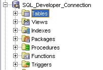
Figure 6: Tables node in the Oracle SQL Developer Connections Navigator

To view the details of any of your tables, expand the Tables node by clicking the plus sign and then double-clicking the individual table name. Figure 7 shows the result of double-clicking the EMPLOYEE table in the Connections Navigator. The table’s column names are displayed vertically in the Connections Navigator pane, and several tabs that provide details about the table are displayed to the right of that pane.

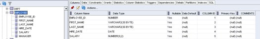
Figure 7: Column list and detail tabs of the EMPLOYEE table in Oracle SQL Developer

By default, the Columns tab is displayed first. It lists the table’s column names and datatypes. It also shows which columns allow null values (that is, the absence of a value), which column or columns are defined as the table’s primary key, and any column comments. (You can see that no primary key has been defined for the EMPLOYEE table in Figure 7. You’ll learn how to create a primary key later in this article series.)

Every column has a datatype, chosen during physical modeling and defined when the table was created. For example, the datatype for the SALARY column in the EMPLOYEE table is NUMBER. Any column defined with the NUMBER datatype permits only numeric data. No text and no alpha characters such as monetary symbols may be stored in a column defined with this datatype. Note that the SALARY column’s datatype is defined as NUMBER(9, 2). The first number in the parentheses (9 in this example) is referred to as the precision, and the second number (2 in this example) is known as the scale. This precision and this scale mean that the SALARY column can have a maximum of nine digits, with a maximum of two digits after the decimal point (useful for columns containing monetary data). If a value with more than two digits after the decimal point is inserted into the SALARY column, no error will occur; the value will simply be automatically rounded by the Oracle Database server.

As you might have guessed, columns defined with the VARCHAR2 datatype store variable-length alphanumeric data (including text, numbers, and special characters). The maximum length of the data is specified in the parentheses. VARCHAR2 is the most commonly used datatype and can store up to 4,000 bytes. In contrast, the CHAR datatype (not shown in Figure 7) allows for fixed-length alphanumeric data only and stores a maximum of 2,000 bytes. I recommend choosing VARCHAR2 over CHAR when you select an alphanumeric datatype to define text columns. With VARCHAR2, particularly if you choose an appropriate maximum length for your columns, you won’t waste storage space. (Choosing a maximum of 4,000 bytes makes sense only if you truly believe that your column will ever contain data values that reach that size limit.) CHAR can waste storage space, because the data is always padded with blank space to the specified fixed length before it is stored.

It’s a good idea to familiarize yourself with multiple data access tools so that you can decide which one works best for you—and so that you can access Oracle Database data in settings (such as a client site, if you are a consultant) where your preferred tool might not be available. SQL*Plus—a command-line-based utility that’s the tool of choice for many old-school Oracle Database programmers and DBAs—is always available, because it is included with every Oracle Database installation. When invoked, the SQL*Plus environment looks like the output shown in Figure 8.

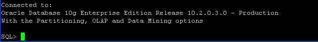
Figure 8: SQL*Plus environment immediately after login

To view a table’s columns and each column’s datatype in SQL*Plus, you use the DESCRIBE command (desc for short), as shown in Figure 9.

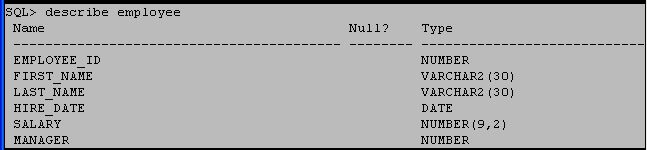
Figure 9: Output of the DESCRIBE command in SQL*Plus

If you’re using Oracle Application Express, you can use any data access tool you’d like, but Oracle Application Express does have its own built-in data access functionality, called SQL Workshop. SQL Workshop contains several subutilities. One of them is the Object Browser, which behaves similarly to the Connections Navigator in Oracle SQL Developer. Double-clicking a table name in a list displays the details for that table in the right-hand pane. Figure 10 shows the output for the EMPLOYEE table and column details displayed in SQL Workshop.

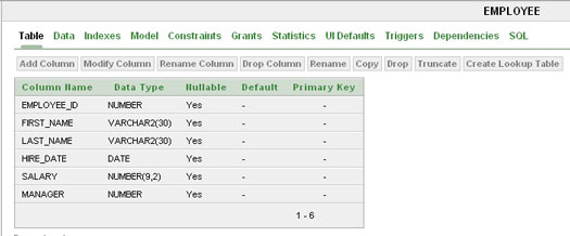
Figure 10: Output of the EMPLOYEE table’s details in Oracle Application Express’ SQL Workshop

Analyzing requirements, planning how data entities should relate to one another, and modeling those entities and their relationships both logically and physically are all essential steps in database design. Knowing your users’ business needs can help you create meaningful entities and relationships and define appropriate attributes with reasonably sized, well-chosen datatypes. Once you’ve defined and created your physical tables, you have many data access options to choose from, including the three no-cost tools from Oracle you’ve learned about in this article.

The next installment of SQL 101 will look at the anatomy of a SQL SELECT statement and explain how to use multiple data access tools to construct SQL statements.

READ more about relational database design and concepts
Oracle Database Concepts 11g Release 2 (11.2)
Oracle Database SQL Language Reference 11g Release 1 (11.1)
Oracle SQL Developer User’s Guide Release 2.1

READ SQL 101 Part 1